Turing Patterns in NumPy

In The Chemical Basis of Morphogenesis (1952), Alan Turing explored the mathematical foundations of the development of living organisms. In particular, he focused on the curious patterns that appear in living organisms. While his most well-known models used differential equations similar to models from fluid dynamics, Turing discovered that “dappled” patterns could be produced by a closed-form equation with the help of a randomized matrix $U \in \{-1, 1\}^{r \times s}$: $$ f(x, y) = \sum{U_{r,s}} \exp \bigg(-\frac{1}{2}\big((x - hr)^2 + (y - hs)^2\big)\bigg)$$ Below is the result Turing obtained using a value of $h = 0.7$.

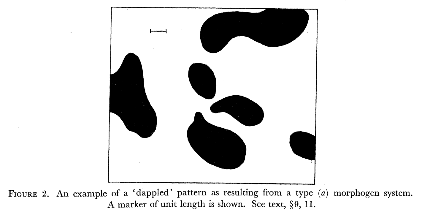
What is most surprising is that this computation was performed by hand over the course of “several hours”, without the aid of a computer. The computation itself is deceptively complex, running in $\mathcal{O}(n^2rs)$ time. With a rather naive NumPy implementation (using apply_along_axis), even moderately sized images took several seconds to generate.

I thought I could do better, so I tried rewriting the code using only vectorized operations. I was able to do this by tiling the $U$, $X$, and $Y$ matrices to obtain 4-D arrays and permuting the axes to perform the computation all at once. This approach proved to be somewhat faster, but at the cost of extreme memory consumption (enough to crash the kernel given sufficiently large matrices!)

def turingVectorized(h=0.7, maxVal=10):
    U = np.sign(np.random.randn(2*maxVal, 2*maxVal))
    x = np.linspace(0, maxVal, 1000)
    X, Y = np.meshgrid(x, x)

    UTile = np.tile(U, (*X.shape, 1,1))
    UTile = np.moveaxis(UTile, [0,1,2,3], [2,3,0,1])
    XTile = np.tile(X, (*U.shape, 1, 1))
    YTile = np.tile(Y, (*U.shape, 1, 1))

    R, S = np.mgrid[:U.shape[0],:U.shape[1]]
    RTile = np.tile(R, (*X.shape, 1, 1))
    RTile = np.moveaxis(RTile, [0,1,2,3], [2,3,0,1])
    STile = np.tile(S, (*X.shape, 1, 1))
    STile = np.moveaxis(STile, [0,1,2,3], [2,3,0,1])

    Z = UTile * np.exp(-1/2 * ((XTile - h*RTile)**2 + (YTile - h*STile)**2))
    Z = np.sum(Z, axis=(0,1))
    return (np.sign(Z)+1)/2

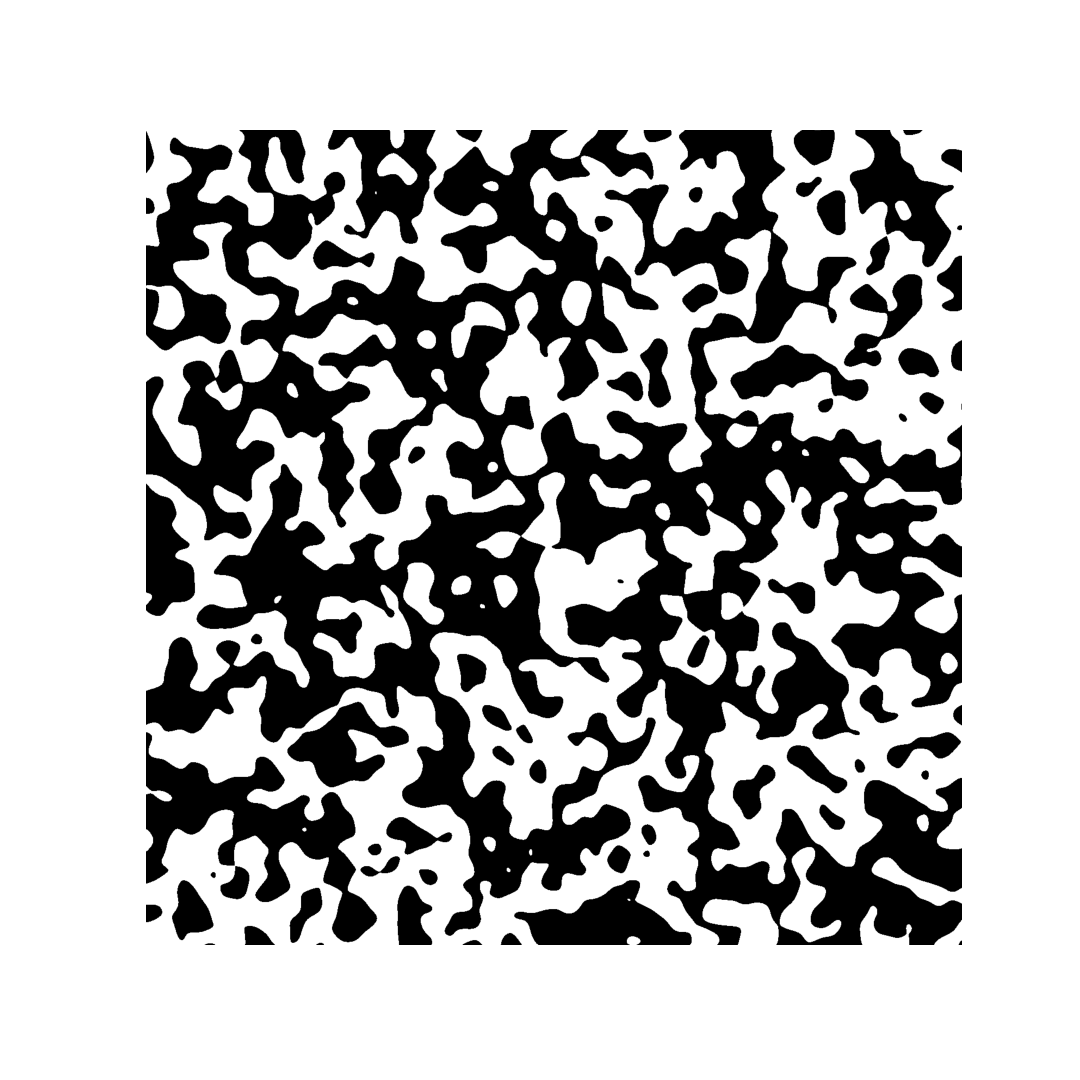
My experiments revealed that the matrix $U$ needed to be approximately 50 percent larger than the maximum $x$ and $y$ values to avoid artifacts at the edges of the image. Sufficiently large values for $r$, $s$, $x$, and $y$ yielded a pattern resembling the cover of a composition notebook: